Research summary

Multi-Modal Open Surveillance with AI-Driven Calibrated Inference

MOSAIC fuses three public, authentication-free surveillance streams, CDC NWSS wastewater, Nextstrain genomics, and WHO DON / ProMED outbreak text, into one calibrated quantity: P(R_t > 1), the probability that transmission is currently growing. The paper gives the full probabilistic model (renewal latent incidence with negative-binomial, Poisson, and Dirichlet-multinomial observation kernels; Poisson-Gamma BOCPD; Jensen-Shannon genomic anomaly; EpiEstim R_t; a noisy-or fusion that reduces to a hierarchical NUTS posterior) and then evaluates the deployed system on real data. Every figure below is computed from real public data, nothing is synthetic.

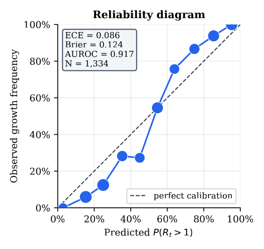
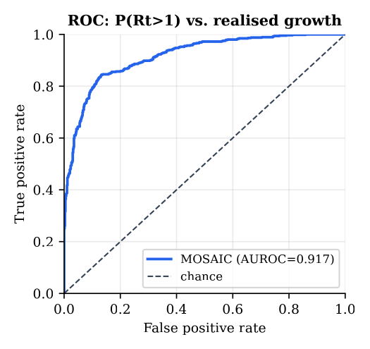
1· The stated probability is calibrated and discriminative

I treat P(R_t > 1) as a probabilistic forecast and ask whether it matches reality. At each day I compute the EpiEstim renewal posterior from data up to that day and check whether wastewater activity actually rose over the following 14 days, a strictly prospective test with no leakage. Across 1,334 day-ahead forecasts on the multi-year national NWSS record the reliability curve hugs the diagonal (ECE 0.086) and the forecast is strongly discriminative (AUROC 0.917). A Murphy decomposition of the Brier score, 0.124 = reliability 0.010 − resolution 0.136 + uncertainty 0.250, confirms both: a tiny reliability term (good calibration) and a large resolution term (the forecasts carry real information about which days grow).

Concretely: when MOSAIC says 75%, activity rises about 87% of the time; when it says 15%, about 6%. That is the empirical meaning of the percentage shown on the dashboard, and it is what lets a user pick an alert threshold and know what it means, which an uncalibrated score cannot support.

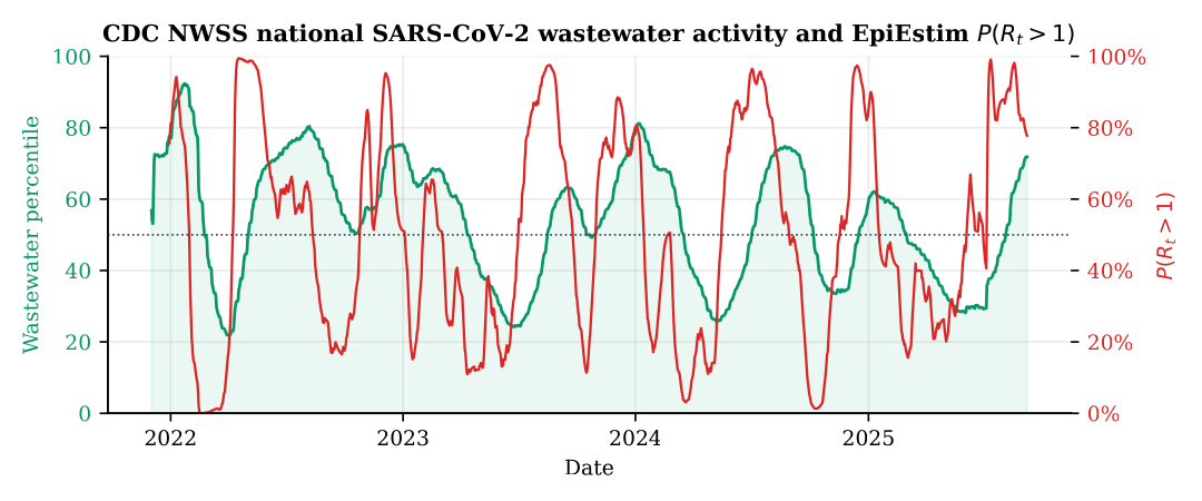
2· It is a leading indicator: ~68 days before the wave peak

Because P(R_t > 1) is a derivative-like signal, it turns at the onset of a wave, long before the level peaks. Detecting national wave peaks and finding the last upward crossing of P(R_t>1) through 50% before each, the growth probability leads the peak by a median of 68 days (mean 73, IQR 67-77). Wastewater is a near-real-time census of community prevalence, shedding starts early and is independent of testing behaviour, and the renewal estimator converts that level into a statement about its slope, crossing 50% before each NWSS wave peaks and dropping below it before each decline.

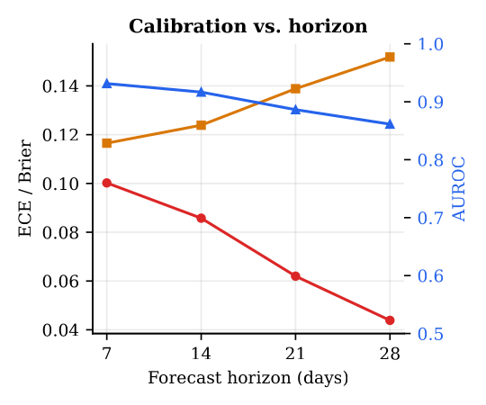
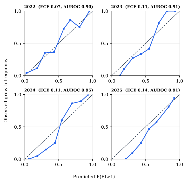
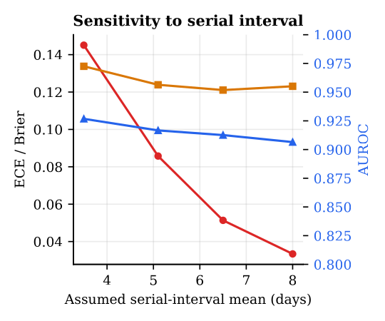
3· The result is robust, across horizons, years, and serial intervals

The calibration is not an artefact of one favourable choice. Sweeping the forecast horizon (7-28 days) reveals a clean trade-off: longer horizons are easier to calibrate (ECE 0.100→0.044) but harder to discriminate (AUROC 0.931→0.861), with 14 days near the knee. Computing the metrics per calendar year (2022-2025), the ECE stays in 0.069-0.145 and AUROC in 0.900-0.947 across the Delta, Omicron, and post-Omicron eras. And varying the assumed serial interval (3.5-8 days) leaves discrimination essentially invariant while shifting calibration smoothly, the literature value (5.1 d) sits in the well-calibrated middle.

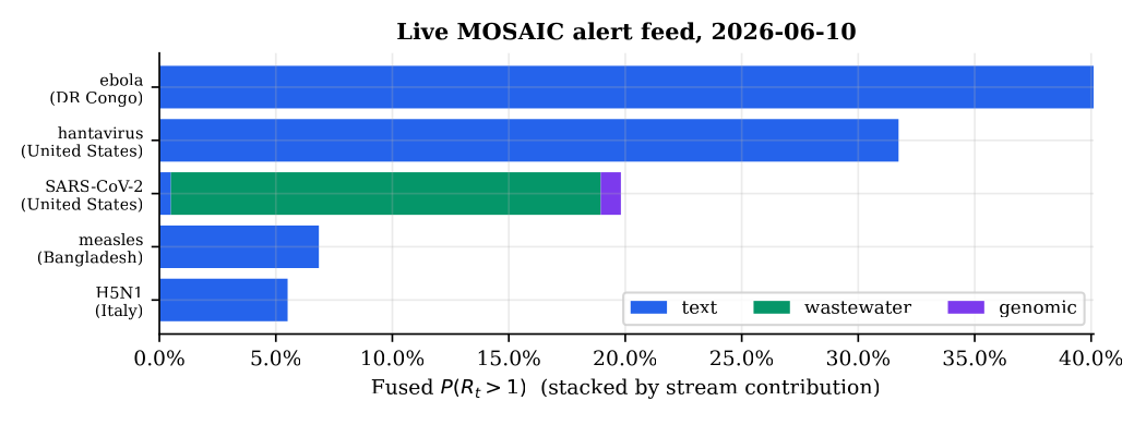
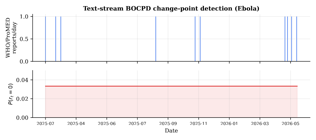
4· Fusion surfaces concurrent outbreaks with per-stream attribution

The independent-evidence (noisy-or) fusion renormalizes weights over the streams that actually carry data for a pathogen, so a text-only outbreak (a filovirus with no wastewater or genomic panel) is not diluted by absent streams. On the live feed the system ranks concurrent real outbreaks, Bundibugyo ebolavirus (DR Congo, Uganda, Sudan), hantavirus clusters, an elevated U.S. SARS-CoV-2 wastewater wave, measles, avian influenza, and lists the specific countries each touches, attributing each alert to its driving stream. The SARS-CoV-2 alert is wastewater-driven; the rest are text-driven, and BOCPD on the report stream spikes when clustered reports follow a quiet period.

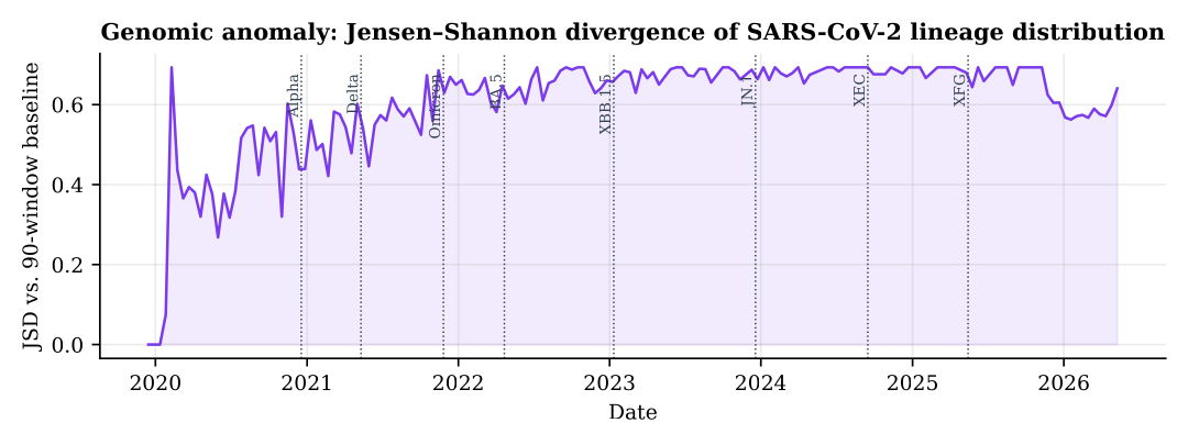
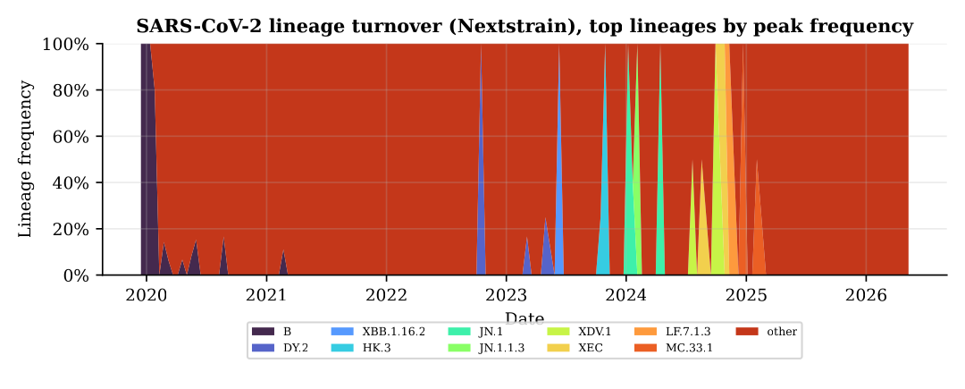
5· Genomic anomaly tracks real variant turnover

The Jensen-Shannon divergence of the SARS-CoV-2 lineage distribution against a rolling baseline rises during documented antigenic transitions (the Omicron sweep, BA.5, XBB, JN.1) and is quiescent when composition is stable. The genomic stream is highly informative about antigenic change but, unlike wastewater, its alarm is not on its own a calibrated probability of growth, which is exactly why the multi-modal design is warranted and why I calibrate on wastewater and treat genomics as corroborating evidence. A pre-computation fix reduces the detector from O(T²K²), billions of operations that timed out on serverless infrastructure, to O(TBK) (~20 ms).

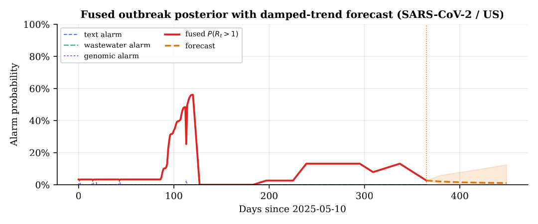
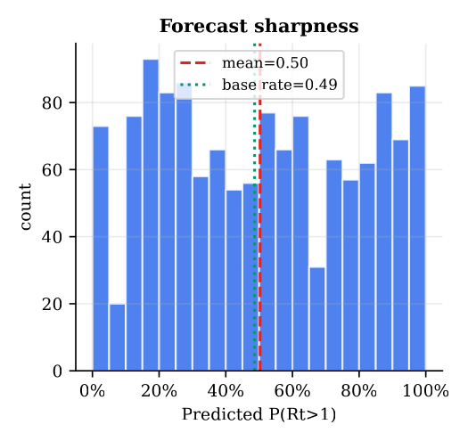
6· Forecasting, and a numerical correction worth flagging

A damped-trend logit-space projection extends the fused posterior forward with a √h-widening 95% band, a deliberately conservative, mean-reverting baseline. Separately, building the backend-free tier surfaced a numerical pitfall worth flagging: the reproduction-number tail probability P(R_t > 1) silently returns wrong values for large-count series when the regularized incomplete-gamma expansion is truncated, it can invert the sign of the estimate. A Wilson-Hilferty normal branch for large posterior shape restores correctness (and reproduces a SciPy reference to three decimals). The sharpness histogram below shows the forecasts are bimodal and their mean matches the base rate.